
Time Series Foundation Models: What They Are and When to Use Them

What is a time series foundation model?
Time series forecasting lies at the heart of many industrial problems, from sales forecasting (airplane ticket sales, Walmart store sales), to demand forecasting (electricity demand, visits to the emergency room), to weather forecasting, and more. It is a classical subject with many decades of accumulated knowledge, historically studied from the point of view of statistics and econometrics. Like language and vision, it has not escaped the deep learning revolution, even if it has not captured the imagination of the general public in the same way.
One important direction in machine learning for time series over the past few years has been the development of Time Series Foundation Models (TSFMs). To give you a sense of the speed at which the field is changing, just over the past 6 months we had the release of Toto 2.0 in May, TiRex-2 in July, TimesFM-3 in August, and t0-beta last week, all 4 in the top-5 of the fev-bench leaderboard, both in point and probabilistic forecasting (for Toto 2.0 only the 2.5B version is in the top-5). In other words, if you last checked the leaderboard 6 months ago, then today you would only recognize Chronos-2 as having kept its place in the top-5.
These models represent a significant shift in how forecasts are produced. Local learning algorithms fit a model (e.g. ETS, ARIMA) to each target time series separately. Global learning algorithms fit a model (e.g. LightGBM, DeepAR) once to a collection of time series of interest, in the hope that the trained model will be good at forecasting series in that collection. TSFMs take this "globality" to the extreme, pretraining on large and diverse collections of time series, and then producing forecasts on new datasets with no further training.
Are all TSFMs the same?
Not at all. They differ in many ways, including the underlying model architecture, model size and licensing restrictions. Crucially for real-world applications, TSFMs differ in their support for including covariates and for probabilistic forecasting.
Covariates
In time series forecasting, a covariate is just extra information we would like to use when forecasting a target time series. For example, when trying to forecast how many people will use the London metro tomorrow, it is a very good idea to use the day of the week as a covariate.
Covariates can be static, such as the location of each weather station; can be dynamic but known only up to the present, such as the demand for electricity when trying to forecast its price; or can be dynamic and known for some time into the future, such as the day of the week or public holidays.
While covariates are widely used in practice, many TSFMs were trained exclusively as univariate forecasting models, such as the original TiRex, Moirai 2.0 or the original Toto, meaning they ignore covariates and use only the history of the target variable when forecasting its future values. In a highly competitive environment, where progress is often measured by benchmark performance, the lack of tasks with covariates in existing benchmarks (e.g. the Monash Time Series Forecasting Archive, GIFT-Eval or TIME) may be partly to blame for this.
This is one of the points made by the fev-bench preprint. The authors created a benchmark where 46 of 100 tasks include covariates, and found significant performance improvements (see fev-bench preprint, Figure 2) by including covariates for the models that support them, which at the time were Chronos-2 and TabPFN-TS.
We are likely to see newer models moving in this direction. At the time of writing, of the models in the top-5 of the fev-bench leaderboard, only Toto 2.0 does not natively support covariates.
Probabilistic forecasting
Often we need not just an estimate of some quantity of interest but also some notion of how uncertain that estimate is. If you provide oxygen to a hospital it is not enough to know that tomorrow the oxygen tank is likely to end the day at 20% of capacity. You need to know that the likelihood the tank will become empty is extremely small. In forecasting, instead of producing only best estimates (point forecasts), we ask for best estimates plus uncertainty quantification (probabilistic forecasts).
TSFMs take different approaches here. TimeGPT-1 is a closed model, but according to the preprint that accompanied its release, it uses conformal prediction to produce prediction intervals, a method that adds uncertainty quantification on top of point estimates under certain assumptions on the data. TabPFN-TS-3.5 turns the time series forecasting problem into a tabular regression problem, where the features include the original covariates but also calendar and generated seasonal features, before asking the tabular foundation model TabPFN-3.5 directly for a probability distribution over the target values.
However, most TSFMs now use the pinball loss to train a quantile regression head to predict a fixed set of quantiles per horizon step. Some, like TimesFM-3, only support 9 quantiles (0.1, 0.2, ..., 0.9), from which you can extract up to 80% prediction intervals. Some allow for more, like TiRex-2, which was trained on 99 quantiles, allowing up to 98% prediction intervals.
Architecture, size, licenses
Most TSFMs, like most language models, are based on the transformer architecture. Of these, there are examples of decoder-only models (e.g. TimesFM-3), of encoder-decoder models (e.g. Chronos Bolt), and encoder-only models (e.g. Chronos-2). A notable exception to the ubiquity of the transformer is TiRex-2, which is based on the recurrent xLSTM architecture.
Parameter sizes span multiple orders of magnitude. Just in fev-bench's top-5 we see models ranging from 82.5M parameters for TiRex-2 (only 38.4M active in univariate mode), to 2.5B parameters for Toto-2.0-2.5B. If we look beyond the top-5, then we can find even smaller models like Toto-2.0-4M at 4M (Toto 2.0 is a family of 5 models of different sizes) or TTM-R3 at 1.4M.
Finally, one important factor to consider when selecting one of these models to put into production is the license under which it is available. Luckily, many of the best models are available under Apache 2.0, a permissive license that in particular allows for commercial use. Important exceptions to this include TimesFM-3, the first model in the TimesFM family to be released under a non-commercial license, Moirai 2.0 and TabPFN-TS-3.5, each under its own non-commercial license.
| Model | Size | Dynamic covariates | Probabilistic | Architecture | License |
|---|---|---|---|---|---|
| TimesFM-3 | 330M | Both (past-only and future-known) | Quantile head, 9 quantiles (0.1, ..., 0.9) | Decoder-only transformer | TimesFM Non-Commercial License v1.0 |
| Chronos-2 | 120M | Both (past-only and future-known) | Quantile head, 21 quantiles (0.01, 0.05, 0.1, ..., 0.9, 0.95, 0.99) | Encoder-only transformer | Apache-2.0 |
| t0-beta | 256M | Both (past-only and future-known) | Quantile head, 21 quantiles (0.01, 0.05, 0.1, ..., 0.9, 0.95, 0.99) | Decoder-only transformer | Apache-2.0 |
| TiRex-2 | 82.5M (38.4M active in univariate mode) | Both (past-only and future-known) | Quantile head, preprint says trained on 99 quantiles, HF checkpoint shows 9 quantiles | xLSTM | Apache-2.0 |
| Toto-2.0-2.5B | 2.5B | None | Quantile head, 9 quantiles (0.1, ..., 0.9) | Decoder-only transformer | Apache-2.0 |
Table 1. Top-5 models in the fev-bench leaderboard at the time of writing and some of their main features.
Should you always use a TSFM?
Not quite. These pretrained models open up new possibilities in terms of reducing time-to-first-forecast. Of course, the usual baselines (Naive, Seasonal Naive, Drift) and the automatic versions of classical methods (AutoARIMA, AutoETS, AutoTheta) are also quite fast to test on new data, but one conclusion to draw from the benchmarks is that, on average, these baselines now lose to several TSFMs.
Besides speed of implementation, there is also the question of how many time series you actually care about. Many companies are deeply impacted by the day-ahead price of electricity in the country where they operate. If they operate in just one country, then this is a single, public time series, and it is quite plausible that domain knowledge and experimentation may lead to a task-specific model that performs better than any TSFM on this time series.
On the other hand, if you are interested in tens, hundreds or thousands of time series, like Walmart forecasting sales per product, then you cannot spend much time and effort studying the properties of each time series. In that case it may be hard to beat a global model like a TSFM.
To illustrate the fact that there is no one-size-fits-all approach, let's look at a concrete example from the fev-bench benchmark. At the time of writing, the live fev-bench leaderboard shows TimesFM-3 at the top and Drift at the bottom, sorted by descending average win rate with respect to the Mean Absolute Scaled Error (MASE) metric. The average win rate of a model is the probability that it outperforms another randomly chosen model on a randomly chosen task (from the models and tasks considered by the benchmark). TimesFM-3 shows up with an 84.6% average win rate, where Drift scores 11.9% (these values will change as new models are added to the leaderboard). But this means that in about 1 out of 10 times, Drift still wins against a random model on a random task.
Figure 1 shows one window of the epf_fr fev-bench task, which tracks the hourly day-ahead price of electricity in France (like most of Europe, this price now has a 15 minute frequency), together with the predictions made by TimesFM-3 and Drift over a 24-step forecast horizon. It is clear that TimesFM-3 does a much better job here than Drift. More generally, over all 20 evaluation windows in this task, and not just the one displayed, Drift achieves a MASE of 1.177, whereas TimesFM-3 achieves a MASE of 0.417, the best score of all models considered (lower is better).
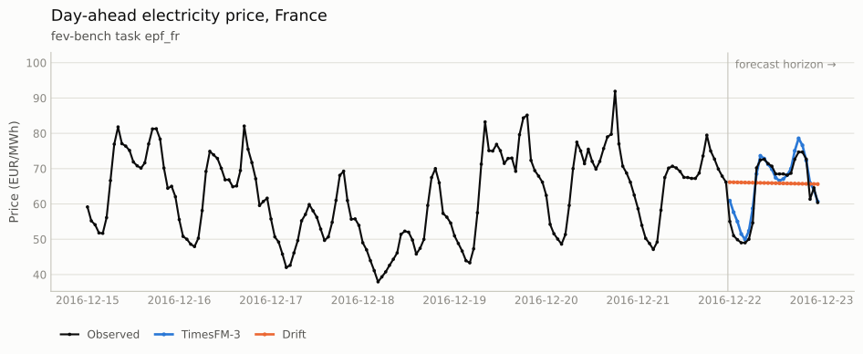
epf_fr task from the fev-bench benchmark, displayed over an 8 day window in December 2016, together with the 1 day forecasts from TimesFM-3 and Drift.However, we can also find tasks where Drift not only does better than TimesFM-3, but actually does better than every other model considered. Figure 2 shows one window of the EU data of the world_tourism task, which counts international tourist arrivals per year, as well as the TimesFM-3 and Drift forecasts over a 5-step forecast horizon. While both models underestimated the growth in international tourist arrivals in the EU over the displayed forecast horizon, the Drift model did a better job than TimesFM-3. Over the 2 windows and 178 series that compose this task (roughly one per country/region), TimesFM-3 scored a MASE of 3.124 and Drift scored a MASE of 2.879, the best score of all models considered.
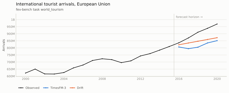
world_tourism task from the fev-bench benchmark, displayed over a 21 year period, together with the 5 year forecasts from TimesFM-3 and Drift.